42 excel line chart axis labels
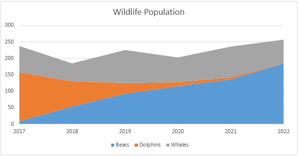
peltiertech.com › add-horizontal-line-to-excel-chartAdd a Horizontal Line to an Excel Chart - Peltier Tech Sep 11, 2018 · The category axis of an area chart works the same as the category axis of a column or line chart, but the default settings are different. Let’s start with the following simple area chart. Notice that the first and last category labels are aligned with the corners of the plot area and the filled area series extends to the sides of the plot area. How to wrap X axis labels in a chart in Excel? When the chart area is not wide enough to show it's X axis labels in Excel, all the axis labels will be rotated and slanted in Excel. Some users may think of wrapping the axis labels and letting them show in more than one line. Actually, there are a couple of tricks to warp X axis labels in a chart in Excel. Wrap X axis labels with adding hard ...
Add or remove data labels in a chart On the Design tab, in the Chart Layouts group, click Add Chart Element, choose Data Labels, and then click None. Click a data label one time to select all data labels in a data series or two times to select just one data label that you want to delete, and then press DELETE. Right-click a data label, and then click Delete.

Excel line chart axis labels
How to Create Line Charts in Excel (In Easy Steps) Line charts are used to display trends over time. Use a line chart if you have text labels, dates or a few numeric labels on the horizontal axis. Use a scatter plot (XY chart) to show scientific XY data. To create a line chart, execute the following steps. 1. Select the range A1:D7. 2. On the Insert tab, in the Charts group, click the Line symbol. spreadsheeto.com › axis-labelsHow To Add Axis Labels In Excel [Step-By-Step Tutorial] Axis labels make Excel charts easier to understand. Microsoft Excel, a powerful spreadsheet software, allows you to store data, make calculations on it, and create stunning graphs and charts out of your data. And on those charts where axes are used, the only chart elements that are present, by default, include: Axes; Chart Title; Grid lines Two-Level Axis Labels (Microsoft Excel) Excel automatically recognizes that you have two rows being used for the X-axis labels, and formats the chart correctly. (See Figure 1.) Since the X-axis labels appear beneath the chart data, the order of the label rows is reversed—exactly as mentioned at the first of this tip. Figure 1. Two-level axis labels are created automatically by Excel.
Excel line chart axis labels. Change axis labels in a chart in Office In charts, axis labels are shown below the horizontal (also known as category) axis, next to the vertical (also known as value) axis, and, in a 3-D chart, next to the depth axis. The chart uses text from your source data for axis labels. To change the label, you can change the text in the source data. Excel Chart not showing SOME X-axis labels - Super User 05.04.2017 · In Excel 2013, select the bar graph or line chart whose axis you're trying to fix. Right click on the chart, select "Format Chart Area..." from the pop up menu. A sidebar will appear on the right side of the screen. On the sidebar, click on "CHART OPTIONS" and select "Horizontal (Category) Axis" from the drop down menu. Four icons will appear ... How to add axis label to chart in Excel? - ExtendOffice You can insert the horizontal axis label by clicking Primary Horizontal Axis Title under the Axis Title drop down, then click Title Below Axis, and a text box will appear at the bottom of the chart, then you can edit and input your title as following screenshots shown. 4. How to rotate axis labels in chart in Excel? Rotate axis labels in chart of Excel 2013 If you are using Microsoft Excel 2013, you can rotate the axis labels with following steps: 1. Go to the chart and right click its axis labels you will rotate, and select the Format Axis from the context menu. 2.
Excel Chart Axis Label Tricks - My Online Training Hub Label specific Excel chart axis dates to avoid clutter and highlight specific points in time using this clever chart label trick. Jitter in Excel Scatter Charts Jitter introduces a small movement to the plotted points, making it easier to read and understand scatter plots particularly when dealing with lots of data. How to Label Axes in Excel: 6 Steps (with Pictures) - wikiHow Select an "Axis Title" box. Click either of the "Axis Title" boxes to place your mouse cursor in it. Enter a title for the axis. Select the "Axis Title" text, type in a new label for the axis, and then click the graph. This will save your title. You can repeat this process for the other axis title. Excel Chart: Horizontal Axis Labels won't update ... I created the data set in Excel 2016, selected the data and inserted a line chart. I sent one line to the secondary axis. The X axis still shows the correct labels. I sent the other line to the secondary axis and brought the first line back to the primary axis. The X axis labels are still correct. In short, I cannot reproduce the problem. support.microsoft.com › en-us › topicPresent your data in a scatter chart or a line chart This is a good example of when not to use a line chart. A line chart distributes category data evenly along a horizontal (category) axis , and distributes all numerical value data along a vertical (value) axis. The particulate y value of 137 (cell B9) and the daily rainfall x value of 1.9 (cell A9) are displayed as separate data points in the ...
Excel tutorial: How to customize axis labels Instead you'll need to open up the Select Data window. Here you'll see the horizontal axis labels listed on the right. Click the edit button to access the label range. It's not obvious, but you can type arbitrary labels separated with commas in this field. So I can just enter A through F. When I click OK, the chart is updated. How to Add Axis Titles in a Microsoft Excel Chart Select the chart and go to the Chart Design tab. Click the Add Chart Element drop-down arrow, move your cursor to Axis Titles, and deselect "Primary Horizontal," "Primary Vertical," or both. In Excel on Windows, you can also click the Chart Elements icon and uncheck the box for Axis Titles to remove them both. Line Chart in Excel (Examples) | How to Create Excel Line Chart? Things to Remember about Line Chart in Excel. Line Chart with a combination of Column Chart gives the best view in excel. Always enable the data labels so that the counts can be seen easily. This helps in the presentation a lot. Recommended Articles. This has been a guide to Line Chart in Excel. Here we discuss how to create a Line Chart in ... Custom Axis Labels and Gridlines in an Excel Chart ... Adding Custom Axis Labels. We will add two series, whose data labels will replace the built-in axis labels. The horizontal axis dummy series (gray line and circle markers) uses the column of numbers (E2:E8) as X values and the column of zeros (F2:F8) as Y values.
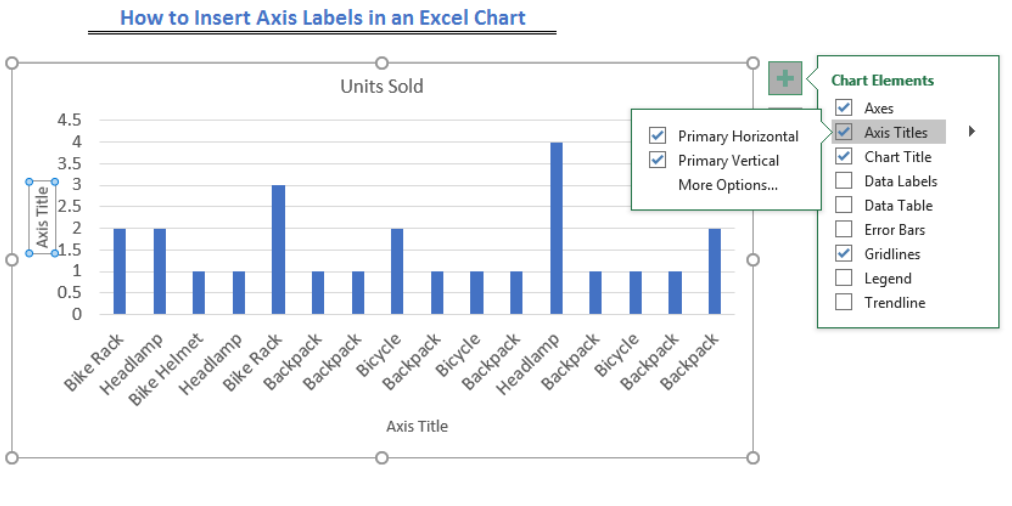
How to Insert Axis Labels In An Excel Chart | Excelchat
Excel charts: add title, customize chart axis, legend and ... Click anywhere within your Excel chart, then click the Chart Elements button and check the Axis Titles box. If you want to display the title only for one axis, either horizontal or vertical, click the arrow next to Axis Titles and clear one of the boxes: Click the axis title box on the chart, and type the text.
32 How To Label Y Axis In Excel - Labels Database 2020
How to display text labels in the X-axis of scatter chart ... Actually, there is no way that can display text labels in the X-axis of scatter chart in Excel, but we can create a line chart and make it look like a scatter chart. 1. Select the data you use, and click Insert > Insert Line & Area Chart > Line with Markers to select a line chart. See screenshot: 2.
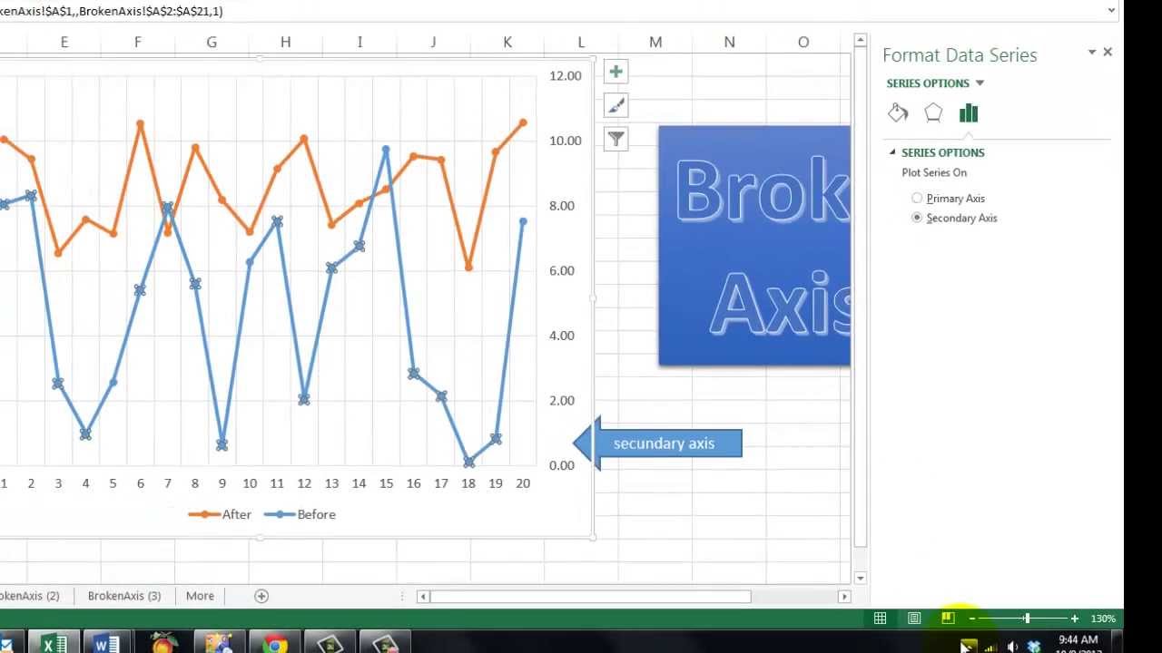
Does Excel Have a Broken Axis? - YouTube
› line-chart-in-excelLine Chart in Excel (Examples) | How to Create Excel ... - EDUCBA Cons of Line Chart in Excel. It can be used only for trend projection, pulse data projections only. Things to Remember about Line Chart in Excel. Line Chart with a combination of Column Chart gives the best view in excel. Always enable the data labels so that the counts can be seen easily. This helps in the presentation a lot. Recommended Articles
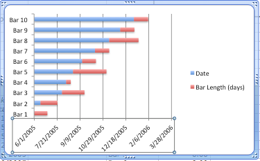
Excel Timelines
EXCEL Charts: Column, Bar, Pie and Line Excel defaults usually lead to a chart that is reasonable but still needs customizing. The general approach is to note that the chart has a number of areas: Chart Title; Plot Area (the actual chart) The x-axis (for charts other than pie chart) which is called a category axis for column or line chart and a value axis for a bar chart.
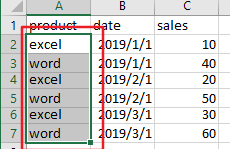
How to Create a Chart with Two-level Axis labels in Excel - Free Excel Tutorial
Excel Chart Vertical Axis Text Labels • My Online Training Hub Click on the top horizontal axis and delete it. Hide the left hand vertical axis: right-click the axis (or double click if you have Excel 2010/13) > Format Axis > Axis Options: Set tick marks and axis labels to None. While you're there set the Minimum to 0, the Maximum to 5, and the Major unit to 1. This is to suit the minimum/maximum values ...
Area Chart in Excel - Easy Excel Tutorial
Excel Charts: Conditionally Highlight Axis Labels on Excel ... Got a Excel Chart question? Use our FREE Excel Help. The below Excel chart highlights the X axis category labels when the monthly data drops below 25. This effect is achieved by using the data labels of 2 extra data series, plotted as lines. Here is the data and formula used to build the chart. The actual data for the column chart is in the ...

How to Add a Third Y-Axis to a Scatter Chart | EngineerExcel
Edit titles or data labels in a chart To edit the contents of a title, click the chart or axis title that you want to change. To edit the contents of a data label, click two times on the data label that you want to change. The first click selects the data labels for the whole data series, and the second click selects the individual data label. Click again to place the title or data ...
Moving X-axis labels at the bottom of the chart below negative values in Excel - PakAccountants.com
How to Format Chart Axis to Percentage in Excel? 28.07.2021 · 3. Click on Insert Line Chart set and select the 2-D line chart. You can also use other charts accordingly. 4. The Line chart will now be displayed. We can observe that the values in the Y-axis are in numeric labels and our goal is to get them in percentage labels. In order to format the axis points from numeric data to percentage data the ...

35 How To Label X And Y Axis In Excel 2013 - Labels For Your Ideas
superuser.com › questions › 1195816Excel Chart not showing SOME X-axis labels - Super User Apr 05, 2017 · In Excel 2013, select the bar graph or line chart whose axis you're trying to fix. Right click on the chart, select "Format Chart Area..." from the pop up menu. A sidebar will appear on the right side of the screen. On the sidebar, click on "CHART OPTIONS" and select "Horizontal (Category) Axis" from the drop down menu.

Individually Formatted Category Axis Labels - Peltier Tech Blog
excelunlocked.com › format-chart-axis-in-excelFormat Chart Axis in Excel – Axis Options Dec 14, 2021 · Thereafter, Axis options and Text options are the two sub panes of the format axis pane. Formatting Chart Axis in Excel – Axis Options : Sub Panes. There is some more sub-division of panes in the axis options named: Fill and Line, Effects, Size and properties, Axis Options. We have worked with the Fill and Line, Effects in our previous blog.

How to Change Horizontal Axis Labels in Excel 2010 - Solve Your Tech
Custom Axis Labels and Gridlines in an Excel Chart 23.07.2013 · Adding Custom Axis Labels. We will add two series, whose data labels will replace the built-in axis labels. The horizontal axis dummy series (gray line and circle markers) uses the column of numbers (E2:E8) as X values and the column of zeros (F2:F8) as Y values.
How to make Excel chart with two y axis, with bar and line chart, dual axis column chart, axis ...
› charts › axis-textChart Axis – Use Text Instead of Numbers – Excel & Google ... Select Data Labels; Click on Arrow and click Left . 4. Double click on each Y Axis line type = in the formula bar and select the cell to reference . 5. Click on the Series and Change the Fill and outline to No Fill . 6. Click on the Original Y Axis Series with numbers and click Delete . Final Graph with Numbers Replaced by Text
Basic Excel Chart Formatting - MS Excel Charting Tutorial Part 4 | Vertical Horizons
How to add Axis Labels (X & Y) in Excel & Google Sheets ... Adding Axis Labels Double Click on your Axis Select Charts & Axis Titles 3. Click on the Axis Title you want to Change (Horizontal or Vertical Axis) 4. Type in your Title Name Axis Labels Provide Clarity Once you change the title for both axes, the user will now better understand the graph.
How to Change Labels for a Chart Axis in Excel 2007
How to Insert Axis Labels In An Excel Chart | Excelchat How to add vertical axis labels in Excel 2016/2013 We will again click on the chart to turn on the Chart Design tab We will go to Chart Design and select Add Chart Element Figure 6 - Insert axis labels in Excel In the drop-down menu, we will click on Axis Titles, and subsequently, select Primary vertical
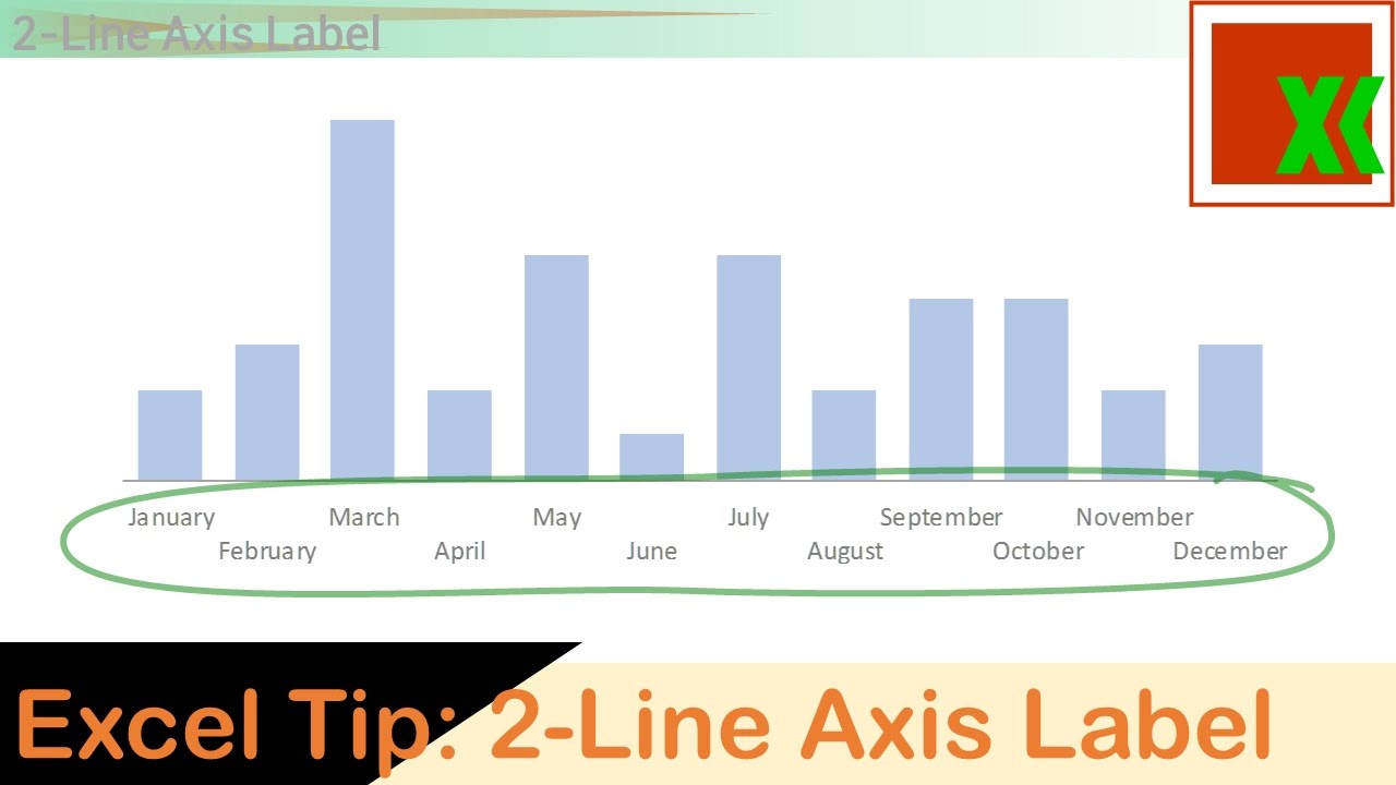
Excel Tip: 2-Line Horizontal Axis Label in Excel Chart - YouTube
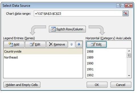
Change axis labels in a chart - support.microsoft.com Right-click the category labels you want to change, and click Select Data. In the Horizontal (Category) Axis Labels box, click Edit. In the Axis label range box, enter the labels you want to use, separated by commas. For example, type Quarter 1,Quarter 2,Quarter 3,Quarter 4. Change the format of text and numbers in labels
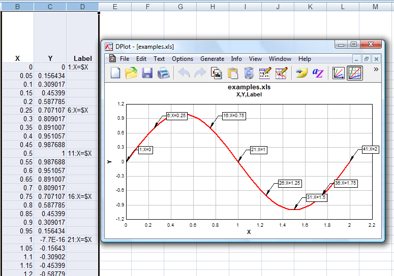
DPlot Windows software for Excel users to create presentation quality graphs
How to Place Labels Directly Through Your Line Graph in ... Select Format Data Labels. In the Format Data Labels editing window, adjust the Label Position. By default the labels appear to the right of each data point. Click on Center so that the labels appear right on top of each point. Umm yeah. So the labels are totally unreadable because they've got a line running through them.
37 Label Axes In Excel 2010 - Modern Labels Ideas 2021
How to wrap X axis labels in a chart in Excel? And you can do as follows: 1. Double click a label cell, and put the cursor at the place where you will break the label. 2. Add a hard return or carriages with pressing the Alt + Enter keys simultaneously. 3. Add hard returns to other label cells which you want the labels wrapped in the chart axis.
Post a Comment for "42 excel line chart axis labels"